If you are analyzing relatively small amounts of data, then your queries won’t cost very much, but if you regularly analyze huge datasets, then your costs can add up quickly. However, with a few adjustments to how you store your data in BigQuery, you can run queries for a fraction of the cost. Partitioning help you manage and query your data with the best possible performance and limit the amount of data that needs to be read when running a query.
Put simply, instead of reading every single record in a table, we will only need to read specific, smaller portions of it – improving both performance and query cost.
Partitioned tables
Table partitioning is a method used to divide tables into chunks, based on attributes in your dataset.

A partitioned table can be created using a partitioning key, or a specific column. There are several ways to partition your table:
- Time-unit column: This method partitions tables based on a time value, such as timestamps or dates.
- Ingestion time: This method partitions tables based on the timestamp at which BigQuery ingests the data.
- Integer range: This method partitions tables based on a numerical value (typically ID’s).
How to apply partitioning to a table
For this example, we will be using date as partition key. Partitioning can only be applied to a table when the table is created, so you cannot add partitioning to an already existing table. You could copy the data from our existing table and put it into a new partitioned table.
You can use the following query to create a partitioned table:
CREATE TABLE projectid.datasetname.tablename

(
  order_id FLOAT64,
  order_date DATE
)

PARTITION BY order_date

OPTIONS(
  require_partition_filter = TRUE
);
For this specific example, I’ve also included the require_partition_filter option in the query. This is a nice safety feature that does not allow for querying the table without specifying order_date. However, it’s important to note that this setting might not be suitable for all use cases. If you frequently need to scan the entire table, or if your queries don’t usually include the partitioned column in the WHERE clause, this setting could be more of a hindrance than a help.

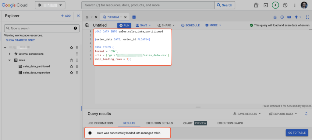
Here is an example of a query for copying data from Cloud Storage to a BigQuery table:
LOAD DATA INTO sales.sales_data

(order_date DATE, order_id FLOAT64)

FROM FILES (
  format = 'CSV',
  uris = ['gs://bucketname/sales_data.csv'],
  skip_leading_rows = 1);
One thing to note is that the LOAD DATA DDL in BigQuery does not recognize headers in CSV files, that’s why we have the skip_leading_rows function. Otherwise it would try to parse header values into data values, leading to an error.

Practical example
I have 2 tables with the exact same data, containing 9994 rows and 2 columns – order id’s and order dates. One of the tables is partitioned by date and the other one is not partitioned at all.
We will execute a simple query to fetch all results from a given date. The number of records received from this query is 6.
SELECT * FROM `projectname.sales.sales_data_partitioned`
WHERE order_date = "2011-08-26"
As illustrated by the screenshots, the partitioned table only searched the specific date partitions requested. In contrast, the unpartitioned table scanned the entire table before limiting the results to the requested date.


For small tables like this, the difference may not be significant. However, when applying this methodology to larger scale operations involving multiple billions of data points, the long-term cost difference between querying an unpartitioned table versus a partitioned one could be substantial.


