Introduction to Pandas DataFrames in Python

Pandas are one of the most powerful and flexible libraries in Python for data analysis and manipulation. I would dare to say it’s an essential library (especially DataFrames) to master when working with data analysis and Python. Provided by the pandas library, DataFrames allow you to store, manage, and analyze structured data with ease. They are particularly well-suited for working with tabular data, such as spreadsheets or SQL tables, and are essential for tasks like code based data cleaning, transformation, and analysis. Whether you’re a data analyst, scientist, or engineer, mastering DataFrames will definitely improve your productivity.

Getting Started with DataFrames

To use DataFrames, you need to have pandas installed. You can install it using pip:

pip install pandas

Next, import pandas into your project:

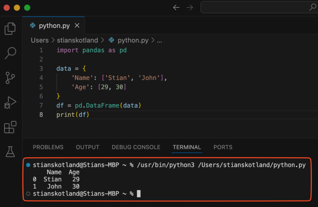
import pandas as pd

You can create a DataFrame from dictionaries or external files. To keep it simple, let’s create the dataset in the code:

data = {
    'Name': ['Stian', 'John'],
    'Age': [29, 30]
}
df = pd.DataFrame(data)
print(df)

If you execute your script, you will now see that your data is available in a familiar tabular format:

Exploring the Dataset

Once your data is loaded into a DataFrame, the next step is to explore it. Pandas offers several methods to quickly understand the structure and content of your dataset. The head() method displays the first five rows, while info() provides a summary of the DataFrame, including column names, data types, and memory usage. To get an overview of numerical columns, you can use the describe() method.

print(df.head())
print(df.info())
print(df.describe())

These commands help you spot inconsistencies, missing values, and potential data quality issues early in your workflow.

Filtering and Querying Data

One of Pandas’ strengths is its ability to filter and query data efficiently. For example, if you want to find all rows where the age is greater than 30, you can write:

very_old = df[df['Age'] > 30]
print(very_old)

This approach is intuitive and avoids the need for complex loops. You can also chain filtering conditions for more refined queries.

Handling missing data is another crucial aspect of data preparation. Pandas makes this process straightforward with methods like dropna() to remove rows with missing values or fillna() to replace them with default values.

df = df.dropna()
df = df.fillna(0)

Understanding how to clean and filter data effectively will save you time and reduce errors in downstream analysis.

Simple Calculations and Conditional Logic

Pandas makes it easy to apply simple calculations and conditional logic across rows and columns. For instance, let’s say you want to add a new column called Age Group that categorizes individuals as either Young or Old based on their age.

df['Age Group'] = df['Age'].apply(lambda x: 'Young' if x < 30 else 'Old')
print(df)

Here, the apply() function evaluates each value in the Age column. If the value is less than 30, the row is labeled as Young; otherwise, it is labeled as Old.

Similarly, you can perform arithmetic operations across entire columns. For example, if you want to calculate an estimated retirement age based on the current age:

df['Retirement Age'] = df['Age'] + 35
print(df)

These examples demonstrate how you can quickly create new insights from your data using simple conditional logic and arithmetic operations.

Grouping and Aggregating Data

Aggregation is also a very common use case, and Pandas simplifies it with the groupby() method. Imagine you want to count the number of people for each age in your dataset. You can group the data by the Age column and apply an aggregation function:

df.groupby('Age').count()

Similarly, you can use the agg() method to apply custom aggregation logic:

df.groupby('Age').agg({'Name': 'count'})

Grouping and aggregation are powerful tools for summarizing and extracting insights from large datasets.

Joining Two DataFrames

In real-world scenarios, you’ll often need to combine data from multiple tables. Pandas makes this straightforward with the merge() function. Let’s say we have two datasets: one containing customer details and another containing their purchase history.

df_customers = pd.DataFrame({'CustomerID': [1, 2], 'Name': ['Stian', 'John']})
df_orders = pd.DataFrame({'CustomerID': [1, 2], 'OrderAmount': [100, 200]})

# Joining on CustomerID
merged_df = pd.merge(df_customers, df_orders, on='CustomerID')
print(merged_df)

This merges the two DataFrames based on the CustomerID column, creating a combined dataset that includes both customer names and their corresponding order amounts.

If you’d like to explore other join types, here are the key options:

Inner Join (default) – Only matching rows from both DataFrames are included.

pd.merge(df_customers, df_orders, on='CustomerID', how='inner')

Left Join – All rows from the left DataFrame are included, with matching rows from the right DataFrame.

pd.merge(df_customers, df_orders, on='CustomerID', how='left')

Right Join – All rows from the right DataFrame are included, with matching rows from the left DataFrame.

pd.merge(df_customers, df_orders, on='CustomerID', how='right')

Outer Join – All rows from both DataFrames are included, with NaN for non-matching rows.

pd.merge(df_customers, df_orders, on='CustomerID', how='outer')

Final Thoughts

These are some very simple examples, but it should give you a good idea of how Pandas helps structure and present data in a readable format. Once you’re comfortable with these basics, you’ll find that Pandas scales seamlessly to handle much larger datasets and more complex transformations. For now, focus on getting familiar with creating, reading, and inspecting DataFrames, as these are the foundations upon which more advanced operations are built.

You can read the official Pandas documentation HERE to get a better understanding of the functions and all the possibilites within this great library.